In a Redshift data warehouse appliance, if two tables use same distribution style and column, then rows for joining columns are on the same data slices. These types of tables are called collocated tables as required data is available in same data slice and less data needs to be moved during query execution. If you join two tables which uses same distribution style and column, then join is called collocated join. In this article, we will check how to optimize the query performance with Redshift collocated tables.
How to Create Redshift Collocated Tables?
Redshift support many data distribution types, If you use KEY distribution, the rows are distributed according to the values in one column of the table. The leader node places matching values on the same node slice. If you distribute a two tables on the same joining keys or columns, the leader node collocates the rows on the slices according to the values in the joining columns so that matching values from the common columns are physically stored together.
Related Articles
- How Redshift Distributes Table Data? Importance of right Distribution Key
- Optimize Redshift Table Design to Improve Performance
Redshift Collocated Table Example
For example, let us take an example of patient and hospital tables, assume that both tables are distributed on patient id. Redshift leader node distributes the rows with the same distribution key to same data slice.
Let’s say, we have inserted sample 5 records of each table. If you verify the table distribution, Redshift should distribute rows with same Patient id to same data slice hence making them collocated tables.
Patient table:
Check patient table data distribution. You can see that data is distributed on to data slices. Here the col = 0 is an id column in the table.
select slice, col, num_values as rows
from svv_diskusage
where name='patients' and col = 0 and rows>0
order by slice, col;

 slice | col | rows
-------+-----+------
     0 |   0 |    3
     1 |   0 |    2
(2 rows)
Hospital table:
Check pat_hospital table data distribution. You can see that data is distributed on to data slices. Here the col = 0 is p_id column in the table.
select slice, col, num_values as rows
from svv_diskusage
where name='pat_hospital' and col = 0 and rows>0
order by slice, col;

 slice | col | rows
-------+-----+------
     0 |   0 |    3
     1 |   0 |    2
(2 rows)
As you can see from both table distribution for same column, data is distributed on the same data slice. So the tables are collocated tables. When you join both tables on first id column, join would be collocated join as required data for computation is available in same data slices.
Verify Redshift Explain Plan for Collocated Tables
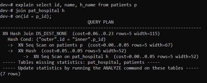
Now let us verify the explain plan for the query joining both tables. There should not be any data distribution.
explain select id, name, h_name from patients p
join pat_hospital h
on(id = p_id);

                                  QUERY PLAN
------------------------------------------------------------------------------
 XN Hash Join DS_DIST_NONE  (cost=0.06..0.23 rows=5 width=115)
   Hash Cond: ("outer".id = "inner".p_id)
   ->  XN Seq Scan on patients p  (cost=0.00..0.05 rows=5 width=67)
   ->  XN Hash  (cost=0.05..0.05 rows=5 width=52)
         ->  XN Seq Scan on pat_hospital h  (cost=0.00..0.05 rows=5 width=52)
 ----- Tables missing statistics: pat_hospital, patients -----
 ----- Update statistics by running the ANALYZE command on these tables -----
(7 rows)
As you can see from explain plan, DS_DIST_NONE, i.e. no data distribution for the given query as required data is available in respective data slices.
Related Article
- Redshift Explain Command and Examples
- Redshift Correlated Subquery and its Restrictions
- How to Choose Correct Compression Encode in Redshift?
- Redshift WHERE Clause with Multiple Columns
Hope this helps 🙂